


In convolutional neural network (CNN),as shown in Figure 1, similarity is calculated on a convolution layer between the input image and the filter. Conventionally, cosine similarity has been used widely to measure the degree of likeness.
Conventional cosine similarity compares the patterns using one-to-one mapping, but the resulting distance metric is highly sensitive to noise, and the distance metric changes in a staircase pattern when a difference occurs between peaks of the input image and the standard image (filter).
As an improvement, we have developed a new convolution (similarity scale) called the “Geometric Distance (GD)” as a superior alternative to cosine similarity.
The GD is more accurate than the conventional cosine similarity in a noisy environment.
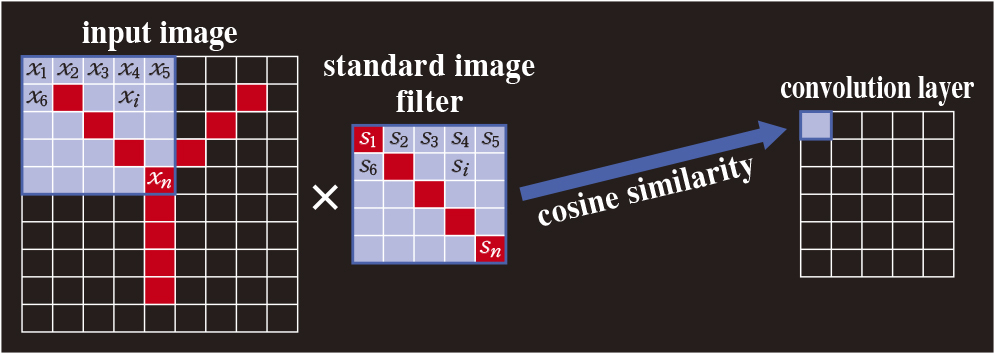
Figure 1 Convolution between input image and filter
Conventional convolution (Cosine similarity):
We create a standard pattern vector s having si (i = 1, 2, …, n) components of the standard image (or sound), and an input pattern vector x having xi (i = 1, 2, …, n) components of the input image (or sound), and represent them as follows.
The cosine similarity is then calculated using the following equation. Note that Figures 2B-5B show the angle θ, which is calculated using an arccosine.

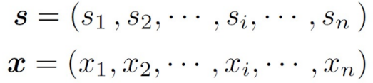
Figure 2A shows an example of the “difference” where the standard sound has two peaks in the spectrogram, and input sounds 1, 2 and 3 have a different position for the first peak. Note that both the standard and input sounds have the same volume.
In Figure 2B, the bar graph on the left shows the cosine similarities θ1, θ2 and θ3 between the standard sound and each of the input sounds 1, 2 and 3. Given that the cosine similarities have the relationship of θ1=θ2=θ3, and therefore, the input sounds 1, 2 and 3 cannot be distinguished from one another.
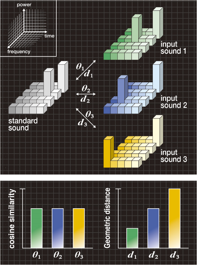
Figure 2A(upper). Typical example of “difference in peak”
Figure 2B(lower). Cosine similarity and geometric distance
Figure 3A shows an example of the “wobble” where the standard sound has a flat spectrogram, input sounds 4 and 5 have the “wobble” on the flat spectrogram, and input sound 6 has a single peak. Each sound is assumed to have variable α, so the standard and input sounds always have the same volume.
In Figure 3B, the bar graph on the left shows the cosine similarities θ4, θ5 and θ6 between the standard sound and each of the input sounds 4, 5 and 6. The cosine similarities have the relationship of θ4=θ5=θ6, and therefore, the input sounds 4, 5 and 6 cannot be distinguished from one another.
Figure 3A(upper). Typical example of “wobble”
Figure 3B(lower). Cosine similarity and geometric distance
Figure 4A shows an example of the “difference in position” where the standard image has a symbol “+”, and input images 1, 2 and 3 have a different position on the horizontal bar.
In Figure 4B, the bar graph on the left shows the cosine similarities θ1, θ2 and θ3 between the standard image and each of the input images 1, 2 and 3. The cosine similarities have the relationship of θ1=θ2=θ3, and therefore, input images 1, 2 and 3 cannot be distinguished from one another.
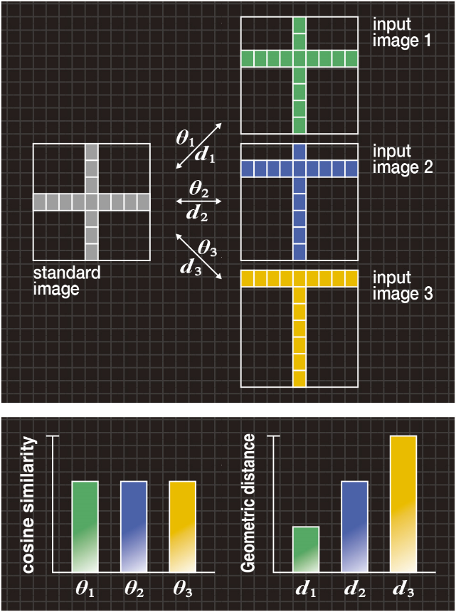
Figure 4A(upper). Typical example of “difference in position”
Figure 4B(lower). Cosine similarity and geometric distance
Figure 5A shows an example of “character deformation” where the standard image has the letter “E” and input images 4, 5 and 6 have the letters “E”, “F” and “G”, respectively.
In Figure 5B, the bar graph on the left shows the cosine similarities θ4, θ5 and θ6 between the standard image and each of the input images 4, 5 and 6. The cosine similarities have the relationship of θ4>θ5>θ6, and therefore, the input letter “E” cannot be recognized correctly.
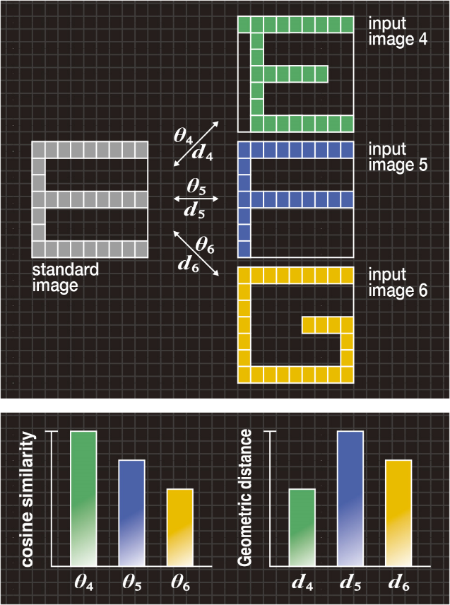
Figure 5A(upper). Typical example of “character deformation”
Figure 5B(lower). Cosine similarity and geometric distance
New convolution (Geometric Distance):
In the GD algorithm, when a “difference” occurs between peaks of the standard and input patterns with a “wobble” due to noise, the “wobble” is absorbed and the distance metric increases monotonically according to the increase of the “difference”.
Bird Call
To authenticate the effectiveness of the GD algorithm, we performed evaluation experiments for the vocalizations of Macleay’s Fig-Parrot. Video shows that, using the GD algorithm, pattern matching even in a noisy environment is accurate.
Concrete (Impact sound)
The same GD algorithm has been successfully used to locate cavities in concrete structures by comparing the acoustic response to controlled surface tapping above integral concrete and concrete compromised by erosion cavities. Recognition accuracy comparing taps arising from integral and cavity-compromised concrete is 17 / 20.
